| Issue |
EPJ Appl. Metamat.
Volume 11, 2024
|
|
|---|---|---|
| Article Number | 5 | |
| Number of page(s) | 14 | |
| DOI | https://doi.org/10.1051/epjam/2024003 | |
| Published online | 08 March 2024 | |
https://doi.org/10.1051/epjam/2024003
Research article
A computational model for generating multihyperuniform distributions for realistic antenna array and metasurface designs
1
School of Electronic Engineering and Computer Science, Queen Mary University of London, London E1 4NS, UK
2
Thales UK, Manor Royal, Crawley, West Sussex RH10 9HA, UK
* e-mail: This email address is being protected from spambots. You need JavaScript enabled to view it.
Received:
9
November
2023
Accepted:
4
January
2024
Published online: 8 March 2024
Abstract
This paper is aimed at studying the concept of multihyperuniformity and applying it to the design of shared-aperture antenna arrays and multi-bit coding metasurfaces. By formulating the theoretical foundation and essential geometric aspects related to this distribution, we create a computational model capable of generating both single hyperuniform and multihyperuniform distributions. Moreover, we put forward specific convergence acceleration techniques that effectively minimize computational time, particularly when dealing with a substantial number of elements. Considering the shape, size, and corresponding geometric constraints of the elements, we generate patterns suitable for practical designs of antenna arrays, as well as metasurfaces. We present an example of a multihyperuniform shared-aperture antenna array as illustration. Specifically, a penta-band circular patch antenna array operating in the C-band with low sidelobes and high realized gain over five different frequency bands is demonstrated. The computational model is also implemented for the design of a multi-bit coding metasurface with scattering reduction attributes.
© O. Christogeorgos et al., Published by EDP Sciences, 2024
 This is an Open Access article distributed under the terms of the Creative Commons Attribution License (https://creativecommons.org/licenses/by/4.0), which permits unrestricted use, distribution, and reproduction in any medium, provided the original work is properly cited.
1 Introduction
The most common arrangement strategy for the antenna elements of arrays or the unit cells of metasurfaces is the periodic distribution, mostly due to its mathematical simplicity. In most cases, the design process is focused on the geometry optimization of the individual elements or unit cells that are employed and no efforts are made to further optimize the resulting designs by employing non-periodic distribution strategies. Nevertheless, it is well known that periodic systems suffer from strong grating lobes when the Bragg condition is met, that is when the inter-element spacing is larger than the operating wavelength. This greatly limits the frequency response of the resulting designs and reduces the design degrees of freedom. Furthermore, when designing multi-bit coding metasurfaces or shared-aperture antenna arrays, the employed elements have different sizes and resonate at different frequencies, while distributed over the same aperture without any element overlaps. It becomes evident that for these scenarios, the use of periodic distributions further decreases the design degrees of freedom and different aperiodic distribution strategies need to be employed.
For the past years, there has been an intensifying interest towards the application of hyperuniform disorder in the fields of antenna array and metasurface design. Hyperuniform disorder is a unique type of distribution that has been found in many natural and biological systems. Such a system is statistically isotropic with no Bragg peaks, like a liquid, while exhibiting suppressed large-scale density fluctuations, like a crystal [1,2]. Hyperuniform distributions have been identified in binary hard-sphere plasmas [3], in packings of Maximally Random Jammed (MRJ) hard-particles [4–6], as well as in non-equilibrium phase transitions of many-particle systems [7–9]. A special type of multi-particle hyperuniform distribution is the multihyperuniform arrangement. Such a distribution is made of different types of particles, with varying sizes, where every different particle distribution, as well as the overall distribution are hyperuniform. This type of multi-particle packing arrangement has been found in the receptor distribution of well-adapted immune systems [10] and in the cone photoreceptor arrangement of avian eye retina [11,12]. Specifically, there exist five different species of photoreceptors on avian eye retina, following a multihyperuniform distribution. As such, birds' vision becomes highly directive and extends to parts of the ultraviolet spectrum.
Due to their unique physical properties, hyperuniform distributions have been extensively applied in different research areas. In the field of material science, materials made of scatterers distributed over a hyperuniform point pattern are shown to be transparent for a broad range of frequencies and directions of incidence [13], whereas in [14] the effective material properties of composite materials where the inclusions follow a hyperuniform distribution are studied. In the field of photonics, hyperuniform distributions are employed to design high-Q optical cavities and bandgaps, as well as free-form photonic waveguides [15–18]. In the field of electromagnetic wave propagation, hyperuniform distributions are employed to overcome the Bragg diffraction limit that is intrinsic to periodic structures. Antenna arrays with hyperuniform disorder have been found to have extraordinary directive emission and scanning features for a wide range of frequencies [19,20], whereas metasurfaces whose unit cells follow a hyperuniform distribution have wide-angle and wideband scattering reduction properties [21].
As it is understood, the growing popularity of hyperuniform distributions for practical applications lead to the need of introducing a computational model that generates hyperuniform distributions for realistic designs of antenna arrays and metasurfaces. Furthermore, it is important to extend this model for multihyperuniform distributions, where the varying shape and size of the elements needs to be taken into account, in order to avoid any element overlaps in the resulting distribution. In this paper, we establish a mathematical model for generating both single and multiple hyperuniform disordered point distributions. Furthermore, we delve into detailed technical discussions surrounding the application of the model to the antenna array and metasurface design process. Lastly, we illustrate how the proposed computational model can be employed in practical examples by presenting a use case study of a multi-band patch array and a multi-bit coding metasurface. As such, this paper's fourfold purpose is: (i) to propose a rigorous and versatile computational model for generating hyperuniform and multihyperuniform distributions of realistic antenna elements and meta-atoms; (ii) to develop methods for rapid convergence acceleration; (iii) to showcase the strength of our method by generating distributions of different types of non-overlapping elements; (iv) to illustrate how a multihyperuniform distribution can be employed for the design of multi-band antenna arrays with broadside directive emission and low sidelobe levels, as well as for metasurfaces with multi-bit coding meta-atoms.
As such, the paper is structured as follows: Section 2 discusses the general properties of hyperuniform distributions and present the fundamental design equations that are associated with these systems. The computational model for generating hyperuniform distributions of circular and square elements along with convergence acceleration methods is proposed in Section 3, where the implementation of our model is also presented along with some example results. Section 4 is dedicated to formulating the computational model for multihyperuniform distributions of circular and square elements, including an example of a penta-band array of circular patches and a scattering reduction metasurface with five different types of meta-atoms. Finally, Section 5 discusses the caveats behind the proposed approach and concludes the work.
2 Hyperuniform point distributions
A hyperuniform point distribution in two-dimensional Euclidean space refers to a configuration of N points where the variance of the number of points  within a spherical sampling window of radius R increases at a slower rate than R2 as R becomes large. Consequently, these systems lack density fluctuations at infinitely long wavelengths, indicating that the structure factor representing the point pattern diminishes near the origin in reciprocal space [1]. The structure factor is a function that is proportional to the scattered intensity of radiation from a system of points and for this reason it is also referred to as the scattering pattern. For a configuration of N points residing within a rectangular area of side lengths Lx,Ly at positions r1, r2, ..., rN, the structure factor is defined as:
 (1)
(1)
where k is an appropriate infinite set of wave vectors. Specifically, on the boundaries of the rectangular computational domain, periodic boundary conditions are applied and the corresponding infinite set of wave vectors in reciprocal space is k = (2πnx/Lx, 2πny/Ly), where nx, ny ∈ ℤ. In order to generate such a distribution in two dimensions we follow the collective coordinate approach as is thoroughly described in Refs. [22,23]. Following this approach, we aim to generate a random point distribution which will be optimized to its ground state. This implies that the total potential energy of the system will be driven to its absolute minimum at or below a chosen cut-off radius in reciprocal space denoted by the letter K. Within this region (0 < |k| ≤ K) the structure factor will be minimized, leading to a special type of hyperuniform disordered distributions which are termed as stealthy [24,25]. Supposing that an N-particle system is distributed over a square aperture with sidelengths Lx = Ly = L, whose area equals to Ω, then the total potential energy of the system is [22]:
 (2)
(2)
In order to quantify the amount of disorder/order in such an N-particle system, each resulting pattern is characterized by the stealthiness parameter χ = M (K)/2N, where M(K) is the number of constrained degrees of freedom which can be determined as follows: Since Φ is minimized for |k| ≤ K*, the goal for the absolute minimum of Φ becomes Φmin = − NM (K)/L2 [23]. Therefore, by considering the minimized potential energy of the hyperuniform system, one can effortlessly determine the number of constrained degrees of freedom based on the square computational domain's sidelength and the number of points in the distribution.
The stealthiness parameter ranges from 0 to 1, with χ = 0 indicating a random structure and χ = 1 a periodic structure. Therefore, the greater the value of χ the more ordered the distribution will be and if χ ≤ 0.5 the distribution is generally considered to belong to the disordered regime of the disorder/order spectrum. As it can be understood, employing the same geometric parameters (i.e., number and size of points and aperture area), but tuning the χ parameter accordingly, will lead to the emergence of different distributions and structure factor patterns. It is important to note that when χ is approximately 0.5, the structure factor is minimized within the circular exclusion region. However, as χ approaches the upper and lower bounds of the order/disorder spectrum, the circular exclusion region gradually disappears. The above observations apply for any particle shape, since the behavior of the structure factor is dependent on the position of the points that are associated with the center of each shape type. Consequently, the structure factor behavior that is described above also applies for the case where combinations of different element shapes are employed in the same distribution. The important thing to note is that the packing fraction needs to be below approximately 60% for any shape type or combination of shape types so that the computational model can converge to hyperuniform solutions while respecting the non-overlapping condition between the elements.
3 Computational model and convergence acceleration methods for generating hyperuniform distributions
The problem of generating a hyperuniform point distribution is essentially a subject of optimization, since we require that the resulting distribution will be such that the objective function of equation (2) is minimized under a specific set of reciprocal and real space constraints. When employing the computational model for the practical design of antenna arrays, we consider the points of the distribution as the centers of two-dimensional elements with a defined shape and size. In the first scenario, each point is treated as the central point of a circle with a designated diameter. Conversely, in the second scenario, each point is treated as the central point of a square. Consequently, the non-overlapping condition needs to be formulated separately for each type of element.
The first step in the process is to define the length of the sides of the square computational area L, as well as the number of points N in the distribution. Then, we define the cut-off radius K and select the range of the wave vectors in reciprocal space (nx,ny) for which the computational model will calculate equation (2). Following the formulation of [22], the cut-off radius K is equal to the square of the reduced distances |ki|/|k1|, where |k1| = 2π/L for the square lattice of k vectors. Therefore, in our model, the constraint for |k| being within the cut-off circle of radius K in the reciprocal space, but excluding the origin, is defined as:


 (3)
(3)
The aim here is to rewrite equation (2) in a form that takes into account the reciprocal space constraint of equation (3). Towards that end, we define the range of the integers nx,ny, denoted as n for which Φ will be calculated. It is crucial to ensure that the range of reciprocal space integers, n, is chosen in such a way that 2n2 > K, as stated in equation (3). This condition ensures that the entire cut-off region lies within the selected range in reciprocal space. Then, the algorithm is constrained to compute the value of Φ only for those nx,ny values for which equation (3) holds, as well as for nx, ny ≠ 0.
Having the aforementioned considerations in mind, we are able to rewrite equation (2) in the form of equation (4), which can be easily implemented with any conventional computational scheme by employing four consecutive iterative processes (one for each sum). In addition, before the start of the third iterative process (the third sum), a conditional function will enforce the reciprocal space constraint, which is formulated in equation (3) with the addition of the requirement for nx, ny ≠ 0. In that way, Φ will only be calculated for those wavevectors that reside within the reciprocal space cut-off region, excluding the origin. A flowchart describing the process for calculating the total potential energy Φ of a system of points, as per equation (4) is illustrated in Figure 1.


 (4)
(4)
The minimization of Φ is realized by employing a constrained gradient descent method, due to its straightforward applicability to the problem and the subsequent non-overlapping constraints that need to be enforced. In order to accelerate the convergence of our algorithm, we formulate the gradient of the objective function with respect to the variables of the system, i.e., the points' coordinates, prior to the initiation of the computational model. Specifically, the gradient is a vector of the following form:
 (5)
(5)
This gradient vector can be easily calculated, bearing in mind that all calculations should be made for the sets of wavevectors k that reside within the cut-off region in the reciprocal space, excluding the origin. As such, it can be easily seen that for a pair of points whose coordinates are denoted as (xi,yi) and (xj,yj), the gradient of the objective function will be:
 (6a)
(6a)
 (6b)
(6b)
 (6c)
(6c)
 (6d)
(6d)
where the first sum indicates that the calculation should be made for those wavevectors that are defined in equation (3). This can be enforced by following the same approach that is described for the formulation of equation (4). A flowchart describing the process for formulating the gradient vector of the total potential energy, as per equations (5) and (6) is illustrated in Figure 2.
Having formulated the objective function Φ as per equation (4), as well as its gradient with respect to the coordinates of points under the reciprocal space constraints (0 < |k| ≤ K), we now turn our attention to the real space constraints that are associated with the geometry of the employed elements in the distribution, as well as the computational domain's boundaries.
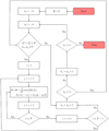 |
Fig. 1 Flowchart describing the process for calculating Φ, as per equation (4). The number of points (N), the square computational domain sidelength (L), the exclusion region radius (K) and the range of the reciprocal space wavevector integers (n) are given by the designer before the start of the process. |
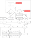 |
Fig. 2 Flowchart describing the process for calculating ∇Φ, as per equations (5) and (6). The number of points (N), the square computational domain sidelength (L), the exclusion region radius (K) and the range of the reciprocal space wavevector integers (n) are given by the designer before the start of the process. |
3.1 Hyperuniform distributions of circular elements
In the case of circular elements we require that all elements reside in their entirety within the computational domain of interest, providing that none of the elements overlap with each other. With N being the number of points in the distribution, we formulate a coordinate vector d of length 2N:
 (7)
(7)
To ensure that all elements remain within the computational domain, it is necessary to establish both a minimum and maximum acceptable value for the coordinates of the points. By positioning the center of the Cartesian coordinate system at the computational domain's midpoint, and assuming that each circular element has a diameter of 2R while the square computational domain has a sidelength of L, we can deduce that the minimum and maximum acceptable values for the coordinate cells in vector d will be -L/2+R and L/2-R, respectively.
The second type of non-linear real space constraint pertains to the inter-element spacing particularly ensuring the absence of any overlapping elements. In order to enforce this, we require that the Euclidean distance ui,j between any pair of points (i,j) in the distribution will be greater than 2R. To implement such a non-linear constraint into our algorithm, we define a constraint vector termed as c(d), which is a function of the coordinate vector of equation (7). We then formulate this vector in such a way that when the non-overlapping constraint is satisfied, c(d) ≤ 0. The rationale behind this choice will be elucidated in subsequent explanations. Due to the requirement ui,j ≥ 2R, the constraint vector c(d) is essentially a function of ui,j. To streamline the calculation of c(d), it is crucial to eliminate unnecessary distance calculations between pairs of points. For instance, if the distance ui,j is already calculated, there is no need to redundantly calculate ui,j. Thus, for the formulation of c(d), the distances between point 1 and all the other N−1 points in the distribution needs to be calculated, then the distances from point 2 to all the other N−2 points in the distribution needs to be calculated and so on. As such, c(d) will be a vector of length N(N−1)/2 of the following form:
 (8)
(8)
where
 (9)
(9)
To further accelerate the convergence, we formulate the gradient of the constraint vector with respect to the points' coordinates, which is a 2N×N(N-1)/2 matrix of the following form:
 (10)
(10)
where c(d)(i) represents the ith element of the constraint vector of equation (8) and d(j) indicates the jth element of the coordinates vector of equation (7). Thus, ∇c (d) will be:
 (11)
(11)
where for a pair of points with coordinates (xi,yi) and (xj,yj), the partial derivatives can be easily calculated as follows:
 (12a)
(12a)
 (12b)
(12b)
 (12c)
(12c)
 (12d)
(12d)
Upon examining equations (11) and (12), it becomes apparent that ∇c (d) forms a sparse matrix, which can be computed efficiently using an iterative process. Specifically, in the first row, N−1 cells are populated with the partial derivatives calculated from equations (12a)−(12d), representing the relationship between the first point and the remaining N−1 points. The remaining cells of the row are filled with zeroes. In the second row, one less calculation is needed as the pair distance between the first and second points has already been computed. This pattern continues for subsequent rows, with the number of required calculations decreasing by one as the pairs of points are considered. By calculating ∇c (d) from top to bottom and row by row, we can fill multiple cells in each iteration. This is possible because ∂ui,j/∂ xi = − ∂ ui,j/∂ xj holds true, allowing for simultaneous calculations. The same process is followed for the bottom half of the matrix, which corresponds to the y coordinates of the points. The flowcharts describing the process for the formulation of the constraint vector c(d) and its gradient matrix ∇c (d) for the case of circular elements are shown in Figures 3 and 4, respectively.
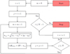 |
Fig. 3 Flowchart describing the process for formulating the non-linear constraint vector c(d) for the case of circular elements, as per equation (8). By c(d)(m), we denote the mth element of the linear constraint vector. The number of points (N) and the diameter (2R) of the circular disks are given by the designer before the start of the process. |
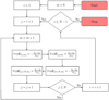 |
Fig. 4 Flowchart describing the process for formulating ∇c (d) for the case of non-overlapping circular elements, as per equations (10)−(12). With ∇c (d) (i,m) we denote the ith cell of the mth row of the non-linear inequality constraint matrix ∇c (d). |
3.2 Hyperuniform distributions of square elements
For the case of non-overlapping square elements, we follow a similar approach to the one presented for the non-overlapping circular disks. Again, the computational domain is a square of sidelength L and the formulation of the objective function to be minimized is as already presented. If we suppose that the squares have a sidelength of 2R, then the requirement for the squares residing within the computational domain is imposed by considering the maximum and minimum acceptable values of the coordinates' vector d as −L/2+R and L/2−R, respectively.
The major difference here lies on the formulation of the non-overlapping condition. Specifically, let us consider the case that is illustrated in Figure 5, where two squares are shown overlapping with each other. The distances between the centers of the squares along the x and y axes are denoted as DSx and DSy, respectively. Since DSx > DSy, it would be more efficient to move the squares along the x axis in order to eliminate the overlap. Thus, for the case of non-overlapping squares the constraint for the distances of the points becomes max(DSx, DSy) ≥ 2R.
Let DSxi,j and DSyi,j represent the center distances along the x and y axes, respectively, between two squares i and j. The constraint vector c(d), of length 2N, is formulated according to equations (8) and (9). In these equations, ui,j is replaced by mi,j, which represents the maximum value between DSxi,j and DSyi,j. The gradient ∇c (d) of the constraint vector is again a sparse 2N × N(N−1)/2 matrix in the form that is shown in equation (11) with ui,j substituted by mi,j. Here, the partial derivatives that populate the constraint gradient matrix can be calculated as follows:
 (13)
(13)
whereas:
 (14)
(14)
The flowcharts describing the process for the formulation of the constraint vector c(d) and its gradient matrix ∇c (d) for the case of square elements are shown in Figures 6 and 7, respectively.
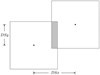 |
Fig. 5 Two overlapping squares. The distances between the centers of the squares along the x and y axes are denoted as DSx and DSy, respectively. Since DSx > DSy, it would be more efficient to move the squares along the x-axis to eliminate the overlap. |
 |
Fig. 6 Flowchart describing the process for formulating the non-linear constraint vector c(d) for the case of square elements. By c(d)(m), we denote the mth element of the linear constraint vector. The number of points (N) and the sidelength (2R) of the squares are given by the designer before the start of the process. |
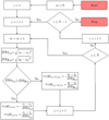 |
Fig. 7 Flowchart describing the process for formulating ∇c (d) for the case of non-overlapping square elements, as per equations(13)−(14). With ∇c (d) (i,m) we denote the ith cell of the mth row of the non-linear inequality constraint matrix ▽c(d). |
3.3 Implementation and numerical results
In order to implement the aforementioned computational model, we use the MATrix LABoratory (MATLAB) environment and specifically the fmincon function, which minimizes an objective function subject to non-linear constraints, by employing a gradient descent method. The official MATLAB guidance for fmincon [26] indicates that the function finds the minimum of a problem specified by:

In our case, the vector x we are seeking corresponds to the coordinate vector d, which represents the distribution points' coordinates, as stated in equation (7). Our aim is to minimize the objective function f(x), which, in this scenario, is the total potential energy of the system Φ defined by equation (4). The vectors lb and ub correspond to the minimum and maximum values of d, respectively, as previously defined. The non-linear inequality constraint function denoted as c(x) takes the coordinate vector d as input. As per the definition of fmincon, the resulting distribution should satisfy c(d) ≤ 0 and this is the rationale behind our choice for the formulation of the non-linear constraint vector. Lastly, fmincon offers the option to predefine the gradient of the objective function and/or the constraint gradient at each iteration of the gradient descent. This avoids the need for numerical calculations and significantly reduces the convergence time, particularly when dealing with a large number of elements.
In the following, for each shape type we generate a stealthy hyperuniform disordered distribution. The distributions all have the same number of points (N = 200) and stealthiness parameter (χ = 0.5) and we choose the same square aperture area sidelength (L = 250 mm) for both cases studied. We choose the diameter of the circles or the sidelength of the squares so that the packing fraction (i.e., the amount of the available space that is occupied by the elements) is around 50% for both cases. It is important to exercise caution when trying to solve such a packing problem and make sure that the packing fraction threshold (≈ 60%) is not surpassed in order to achieve convergence towards feasible hyperuniform solutions. For N number of non-overlapping circles with a diameter of 2R distributed over a square aperture area of sidelength L, the packing fraction in percentage is φcircle = πNR2/L2 × 100, whereas for non-overlapping squares with a sidelength of 2R, the packing fraction in percentage is φsquare = N (2R) 2/L2 × 100.
In order to illustrate the capabilities of our computational model, we specifically consider four use cases,
Case 1: neither the objective function nor the non-linear constraint gradient is defined in advance;
Case 2: only the non-linear constraint gradient is defined in advance;
Case 3: only the objective function gradient is defined in advance;
Case 4: both the objective function and the non-linear constraint gradients are defined in advance;
For both the distribution of circles and squares, we tested our computational model for N = 200 and L = 250 mm. The diameter of the circles is chosen to be equal to 2R = 14 mm, whereas the sidelength of the squares is 2R = 12.5 mm leading to a packing fraction of around 50% for both cases.
The results are depicted in Figure 8, with top and bottom panels showcasing the resulting stealthy hyperuniform disordered distributions of non-overlapping circular and square elements, respectively. From left to right the results are illustrated for Cases 1–4. It should be noted that for all the cases shown, the resulting structure factor is identical, thus proving that more than one distributions can lead to identical reciprocal space behavior, which is also not affected by the element shapes. Furthermore, Table 1 presents a tabulation of the convergence time (Δt) for the computational model, as well as of the percentage decrease in Δt for both cases of circular or square elements, compared to Case 1 and for all the cases shown in Figure 8. As it can be seen, the prior calculation of the objective function gradient (Case 3) has the most significant effect on the decrease of the computational time, whereas the constraint gradient does not alter much the computational time (Case 2). Of course the algorithm convergence time is at its minimal when both gradients are calculated (Case 4). The computer used to run our tests had a 64-bit operating system with 48 GB RAM and a 3 GHz processor.
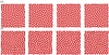 |
Fig. 8 Stealthy hyperuniform disordered distributions for (a) non-overlapping circles and (b) non-overlapping squares. From left to right the distributions correspond to Cases 1–4. |
4 Computational model for generating multihyperuniform distributions
In this section, we formulate the computational model for generating such a distribution for the case of different species of circular elements. Towards that end, we apply the methodology for the single stealthy hyperuniform disordered distribution of circles that was presented in Section 3.1, but the formulation of the non-linear real space constraints needs to be altered. In particular, let us consider that M different species need to be distributed in a stealthy multihyperuniform manner within a square computational domain of sidelength L. Each species consists of Ni particles, where i indicates the ith species in the overall distribution. Thus, for each species the total potential energy Φi , as well as its gradient ∇Φi needs to be separately formulated as per equations (4) and (5).
The species are distributed one-by-one over the computational domain of interest. Thus, for the first species, the process is identical to the one described in Section 3.1, since the computational domain is empty. The subsequent species to be distributed must avoid overlapping with previously placed elements, including those from previous species. Therefore, the non-linear real space constraints need to be redefined to ensure that there is no overlapping between elements of the same species as well as elements from previously distributed species. Towards that end, we term as u(m,n)i,j the Euclidean distance between the ith particle of the mth species, with coordinates (x(m)i, y(m)i) and the jth particle of the nth species with coordinates (x(n)j, y(n)j). Moreover, each species possesses a distinct coordinate vector. For the mth species, the coordinate vector is represented as dm, and its length is 2Nm, where Nm denotes the number of elements belonging to this particular species.
Now the non-overlapping constraint becomes u (m, n) i,j ≥ Rm + Rn, where Rm, Rn are the radii of the circles of the mth and the nth species, respectively. Therefore, for the mth species, the non-overlapping constraint vector  needs to be formulated so that the constraint is imposed for circles of the same species as well as circles of different species.
 (15)
(15)
where, cm(dm) is calculated as per equations (8) and (9) and represents the non-overlapping constraint for circles of the same species. As such, it is a vector of length equal to Nm (Nm − 1)/2. When m ≠ n, the cn (dm) vector represents the non-overlapping constraint between the previously distributed nth species and the mth species that we are looking to distribute. This vector is of length NmNn and is formulated as follows:
 (16)
(16)
where

 (17)
(17)
Therefore the total non-linear non-overlapping constraint vector of equation (15) for the mth species to be distributed is of overall length Nm (Nm − 1)/2 + N1Nm . . . + Nm−1Nm. The next step is to formulate the gradient matrix of the non-linear constraint vector. For the mth species to be distributed, the constraint gradient matrix is denoted as  . It is evident that this matrix is of size 2Nm × [Nm (Nm − 1)/2 + N1Nm + . . . + Nm−1Nm] . The formulation of this matrix is very similar to the formulation for the single species in equation (11), but with N1Nm + . . . + Nm−1Nm columns added on the right side to calculate the partial derivatives for the non-overlapping constraint between the mth species that we want to distribute and the nth species that are already distributed. These derivatives can be easily calculated as follows:
 (18a)
(18a)
 (18b)
(18b)
Finally, the requirement for each element residing in their entirety within the computational domain of interest is formulated with the same manner as for the case of the single stealthy hyperuniform distribution for each of the species that is distributed. In addition, for the case of stealthy multihyperuniform distribution of squares, the process that is followed is very similar to the one presented for the circles, but taking into account the modifications to the non-overlapping constraint vector and its gradient as presented in Section 3.2 for the case of the single stealthy hyperuniform distribution of squares. Consequently, with proper modifications to the non-overlapping conditions, the computational model for multihyperuniform distributions can be employed for the case where a combination of both circular and square elements are distributed over the same aperture area.
4.1 The penta-band multihyperuniform shared-aperture antenna array of circular patches
In order to illustrate the concept, we have employed our computational model to design a penta-band multihyperuniform shared-aperture antenna array of circular patches resonating at 4, 5, 6, 7 and 8 GHz. In Figure 9, the top panel illustrates the resulting hyperuniform patch subarrays, from left to right resonating at 4, 5, 6, 7 and 8 GHz, as well as the multihyperuniform distribution on the rightmost subfigure. The bottom panel illustrates the associated structure factor plots, where it can be seen that each distribution adopts a stealthy hyperuniform reciprocal space behavior, while the overall distribution is also hyperuniform.
Finally, we have simulated the same shared-aperture antenna array by employing the use of Computer Simulation Technology (CST) Microwave Studio. In particular, the patches were designed to resonate at their corresponding frequencies when etched over an FR-4 substrate with a height of h = 0.8 mm and a relative permittivity of εr = 4.3. The radii of circular patch antennas can be calculated based on the formula provided in [27], which resulted in R1=10.1 mm, R2 = 8 mm, R3 = 6.55 mm, R4 = 5.55 mm and R5 = 4.8 mm for the 1st to 5th species, respectively. The patches were excited by employing a probe feeding method, where the probe is situated Ri/3 away from the center of each patch, with Ri being the radius of the ith species patch. A simultaneous excitation method was employed to excite the patches at their corresponding frequencies, while the out-of-band patches were terminated with a 50 Ohm load. The square aperture area's sidelength was defined as L = 350 mm and the overall dimensions of the array can be seen in the top panel of Figure 10. Furthermore, the ϕ = 0° and ϕ = 90° planes are shown, while θ = 0° is situated at the array's boresight. The bottom panel of the same figure illustrates the polar radiation pattern plots when the 1st, 2nd, 3rd, 4th and 5th species are excited at 4, 5, 6, 7 and 8 GHz, respectively (from left to right), where the angular and radial coordinates correspond to the ϕ and θ angles, respectively. It is worth mentioning that in our previous work on hyperuniform disordered arrays [19], a parametric study showed that there exist optimal combinations for the number of elements (N) and stealthiness parameter (χ) for optimal performance in terms of wideband sidelobe suppression and directive beam-steering, where for an increasing number of elements the optimal stealthiness parameter converges towards the middle of the disorder/ order spectrum, i.e., χ ≈ 0.5. Following this analysis, here each subarray consists of 25 circular patches and the stealthiness parameter (χ) is around 0.5 for all cases. Furthermore, in [19], the radius of the exclusion region (θexc) in the angular radiation pattern plot of a hyperuniform disordered array is related to the structure factor cut-off radius (K), the operating wavelength (λ) and the square aperture's sidelength (L) through:
 (19)
(19)
For the case of the penta-band patch array with multihyperuniform disorder, each array has N = 25 elements and χ = 0.5 and thus the cut-off radius is K = 16 for all subarrays. On the other hand, each subarray resonates at different frequencies, namely at 4, 5, 6, 7 and 8 GHz and as such the exclusion region radius for each subarray at its corresponding operating frequency becomes θexc1 ≈ 59°, θexc2 ≈ 43°, θexc3 ≈ 35°, θexc4 ≈ 29° and θexc5 ≈ 25° for the 1st to 5th species, respectively. This is qualitatively verified by observing the bottom panel of Figure 10 where the exclusion region becomes smaller as the operating frequency increases. It is also notable that when the structure factor is calculated, the distribution is considered to be replicated an infinite number of times along its axes and, for this reason, the structure factor values within the exclusion region are absolute zero and a clear circular exclusion region can be seen (Fig. 9). On the other hand, when these distributions are implemented in an array of finite dimensions, the effects of the square computational domain can be seen in the radiation pattern of the subarrays, where the diffraction pattern of a square aperture can be seen within the exclusion region [19]. Nevertheless, the radiation values within the exclusion region are very low compared to the main lobe, as well as the peak sidelobes.
Furthermore, the simulated frequency response of the multihyperuniform array of circular patches shown in the top panel of Figure 10, with respect to the peak far-field realized gain and sidelobe levels is illustrated in Figure 11, where the dotted vertical lines indicate the transition between operating bandwidths of consecutive species. Furthermore, in the same figure, two types of simulation results are given, that is the isolated case of each species in the physical absence of the rest of the species (Isolated HuD) and the multihyperuniform (multi-HuD) results corresponding to the performance of each species but with the physical presence of the out-of-band elements, when the latter have their excitation ports terminated to 50 Ohm loads.
As it can be seen, the peak far-field realized gain and side lobes are unaffected by the presence of the out-of-band elements, with the maximum gain of 16.6 dBi observed at 8 GHz. The side lobes remain below -10 dB for most of the operating frequencies and for both orthogonal planes, with a maximum observed value of -9.6 dB at 6.5 GHz. Lastly, it is worth noting that this array has a packing fraction of around 17% and although in many cases the out-of-band elements are in close proximity to the excited elements, the physical presence of the former does not detrimentally deteriorate the performance of the latter.
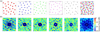 |
Fig. 9 The penta-band multihyperuniform antenna array of circular patches. (a) The hyperuniform patch arrays distributions and the overall multihyperuniform patch array distribution and (b) the corresponding structure factor plots. |
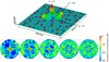 |
Fig. 10 Top: The multihyperuniform penta-band shared-aperture patch antenna array. Bottom: Polar normalized far-field radiation pattern plots. From left to right: 1st species at 4 GHz, 2nd species at 5 GHz, 3rd species at 6 GHz, 4th species at 7 GHz and 5th species at 8 GHz. The angular and radial coordinates correspond to the ϕ and θ angles, respectively. |
 |
Fig. 11 Simulated frequency response of the multi-band shared-aperture patch antenna array with multihyperuniform disorder (multi-HuD) shown in the top panel of Figure 10 compared with the simulated frequency response of the subarrays in the physical absence of the out-of-band elements (Isolated HuD). (a) Peak far-field realized gain and (b) peak side lobe level values. The dotted vertical lines indicate the transition between operating bandwidths of consecutive species. |
4.2 The multihyperuniform disordered scattering reduction metasurface of square meta-atoms
In order to illustrate how the proposed computational model for generating multihyperuniform distributions can be employed for the design of scattering reduction metasurfaces, we employ square metallic patches as the meta-atoms in the distribution. In particular, we consider the square patch that is shown in Figure 12a following the design presented in [28]. Figure 12a illustrates the dimensions of the unit cell, where the patch is backed by a Perfect Electric Conductor (PEC), the employed substrate is FR-4 with relative dielectric permittivity of 4.6 and loss tangent tan δ = 0.001 and its height is h =1 mm. The patch is made of copper with a conductivity of σ = 5.8 × 10⁷ S/m and the periodicity of the unit cell is defined as p =7.5 mm. In order to design the multi-bit coding scattering reduction metasurface with multihyperuniform disorder we employ five different meta-atoms with different sidelength dimension (w) for the patches and simulate their response by employing CST Microwave Studio. The five different selected sidelength dimensions for the patches lead to the reflection phase and amplitude results shown in Figure 12b and Figure 12c, respectively for the five different species of meta-atoms.
In [21] a scattering reduction metasurface with single hyperuniform distribution was designed and it was shown that the Radar Cross Section (RCS) was minimized when the employed hyperuniform distribution is defined to be towards the disordered regime in the disorder/order spectrum. As such, for this work we define the five species to follow a hyperuniform distribution with χ = 0.3. We employ the computational model presented earlier for the square patches distribution, where the square aperture area's sidelength is L = 130 mm and the resulting configurations for the unit cell dimensions presented in Figure 12 can be seen in Figure 13a, while the corresponding structure factor plots are illustrated in Figure 13b. As it can be seen from the corresponding structure factor plots, each species follows a hyperuniform distribution and the overall distribution is hyperuniform as well. Note that when comparing the structure factor plots for the scattering reduction metasurface with the ones for the multi-band shared-aperture array in Figure 9b, the circular exclusion region is smaller and this is due to the different definition of the stealthiness parameter for the different designs. For the shared-aperture array, χ = 0.5 was employed for the species' distribution, in order to lead to unidirectional emission with low sidelobes. For the scattering reduction metasurface design, the species' distributions have χ = 0.3, in order to maximize the RCS reduction. In particular, for smaller values of the stealthiness parameter, the phase gradient in the hyperuniform disordered metasurface becomes more inhomogeneous, leading to larger RCS reduction values compared to a bare metal plate of the same dimensions. Therefore, χ = 0.3 is optimal for such a design and hence the choice for the stealthiness parameter value of the hyperuniform distributions that make up the multihyperuniform scattering reduction metasurface that is presented here.
We proceed with simulating the designed multi-bit coding metasurface with multihyperuniform disorder by employing the use of CST Microwave Studio. In particular, the metasurface is illuminated by a plane wave with linear polarization, incoming from the top of the metasurface. A metallic plate with the same dimensions is also simulated, in order to observe the RCS reduction of the designed metasurface compared to the metallic plate. The radiation RCS pattern results are shown in Figure 14 for the operating frequency of 10.5 GHz. The top panel of Figure 14 shows the three-dimensional normalized RCS radiation pattern results for both the metal plate (left) and the multihyperuniform metasurface (right) and the bottom panel illustrates the normalized RCS radiation pattern results for the yz plane for both the metal plate (black solid line) and the multihyperuniform metasurface (red dotted line). The illustrated results are normalized against the metal plate peak RCS value and the operating frequency is fixed at 10.5 GHz. As it can be seen the multihyperuniform metasurface scatters the incident plane wave towards various directions, due to the different reflection phases of the different species which follow a multihyperuniform distribution. The observed simulated RCS reduction compared to the metal plate of equal dimensions is at −14 dB.
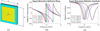 |
Fig. 12 The square meta-atom employed for the multi-bit coding scattering reduction metasurface with multihyperuniform disorder. (a) The square patches are made of copper (σ = 5.8×10⁷ S/m) with varying sidelength w for the different species, the FR-4 substrate's height is h =1 mm with εr= 4.6 and tan δ = 0.001, the periodicity of the unit cell is p =7.5 mm and the patches are backed by a PEC plane. (b) Simulated reflection phase results for varying w for the five different species. (c) Simulated reflection amplitude for varying w for the five different species. |
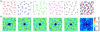 |
Fig. 13 The multi-bit coding scattering reduction metasurface with multihyperuniform of square patches. (a) The hyperuniform patch subarrays distributions and the overall multihyperuniform patch array distribution and (b) the corresponding structure factor plots. |
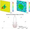 |
Fig. 14 Top: 3D RCS radiation pattern plots for the metallic plate (right) of equal dimensions to the multihyperuniform metasurface (right) at 10.5 GHz. Bottom: The yz plane RCS radiation pattern plots for the metallic plate (black solid line) and the multihyperuniform metasurface (red dotted line) at 10.5 GHz. The RCS values are normalized against the peak RCS value of the bare metallic plate. |
5 Discussion and conclusions
The generation of multihyperuniform distributions for realistic antenna array and metasurface designs is a complex task involving multiple parameters. The number of species, the number of antenna elements or meta-atoms for each species, the size and shape of the elements, and the overall packing fraction all play significant roles in ensuring the algorithm convergence and in determining the computational complexity of the proposed method. It is crucial to select these parameters carefully to ensure that the algorithm converges to viable solutions, specifically multihyperuniform distributions that adhere to the real space constraints. In addition, it is preferable that the species with larger particle sizes are distributed first and that the next species to be added will have smaller element sizes, since less space will be available over the aperture area. Generally, the overall packing fraction should not exceed the threshold of 60% in order for the algorithm to converge to feasible multihyperuniform solutions. However, this threshold is contingent on the size and shape of the particles being utilized. Specifically, higher resonant frequency ratios between different elements will result in higher packing fractions. Furthermore, in the future we aim to generalize the proposed computational model for arbitrary shaped particles and not just circular and square elements as the ones that are employed here.
The array with hyperuniform disorder is an optimized non-periodic distribution which due to the varying inter-element spacing is a sparse design. Compared to the case where a periodic distribution is employed to fill up the same aperture area, the array with hyperuniform disorder is expected to have reduced aperture efficiency, especially as the operating frequency increases and the inter-element spacing becomes large compared to the operating wavelength. On the other hand, the varying inter-element spacing in the hyperuniform disordered array leads to the reduction of the undesired mutual coupling between the elements at low frequencies and to the suppression of the grating lobes at higher frequencies. Furthermore, a hyperuniform array can be employed to reduce the number of elements required to satisfy certain radiation pattern requirements, such as grating lobe suppression and gain levels, compared to an array with periodic distribution. This is also evidenced in [20], where a reflectarray with hyperuniform disorder is found to have the same radiation pattern attributes as that of a periodic reflectarray, but with a 36% decrease to the employed elements, effectively reducing the cost of the overall design. Furthermore, for multi-band shared-aperture arrays, employing periodic distributions greatly decreases the design degrees of freedom and as such the limited available area does not allow for distributing other arrays, while suppressing the grating lobes. As evidenced in this work, the sparse optimized non-periodic distribution of the array with hyperuniform disorder allows for the introduction of several different arrays that operate at other frequency bands, while suppressing the grating lobes and maintaining high realized gain.
The simulation results for the penta-band patch array and the scattering reduction multi-bit coding metasurface serve the purpose of providing some initial insight on the performance of multihyperuniform antenna arrays and multi-bit coding metasurfaces, as well as to illustrate the strength of our computational model and its straightforward applicability to such designs. As a result, the fabrication of the aforementioned multi-band array and multi-bit coding metasurface and the measurement of their performance is beyond the scope of the present paper.
6 Implications and influences
The present paper opens up new possibilities for implementing the concept of hyperuniform and multihyperuniform disorder for designing realistic antenna array and metasurface structures. The proposed method and computational model can be generalized for different shapes and sizes of the employed elements and as such can be applied for various scenarios and at different operating frequencies. As such, the proposed computational model can be applied at various engineering fields, where non-periodic arrangements of different elements can lead to performance enhancement for the problem at hand. As such, it is robust and applicable to different scenarios. We have presented a fast and efficient method for generating hyperuniform and multihyperuniform distributions for realistic antenna array and metasurface designs. Our findings demonstrate that incorporating the gradient of the objective function and of the real space constraints significantly reduces the convergence time of the algorithm by nearly 50%. This reduction is crucial, particularly when dealing with a substantial number of elements. Having formulated the computational model for generating multihyperuniform distributions, we are now able to generate such distributions and apply them in the field of shared-aperture and small/compact antenna arrays, as well as multi-bit coding metasurfaces. This approach opens up the possibility of designing multifunctional multi-band antenna arrays and metasurfaces without the need for complex distribution strategies such as thinning techniques, perforating elements, time-consuming optimization schemes, or sophisticated stacked array designs.
Funding
O. Christogeorgos' research was funded by the Engineering and Physical Sciences Research Council (EPSRC) with project reference number 22720076 and by Thales UK. Y. Hao’s work is partially funded by IET AF Harvey Research Prize, EPSRC (EP/R035393/1, EP/W026732/1, EP/X02542X/1) and the Royal Academy of Engineering. The APC was funded by the School of Electronic Engineering and Computer Science of Queen Mary University of London.
Conflicts of interest
OC has received funding from the Engineering and Physical Sciences Research Council (EPSRC) with project reference number 22720076 and from Thales UK. EO certifies that he has no financial conflicts of interest (eg., consultancies, stock ownership, equity interest, patent/licensing arrangements, etc.) in connection with this article. YH has received funding from the Institute of Engineering and Technology (IET) AF Harvey Research Prize, from the Engineering and Physical Sciences Research Council (EPSRC) with project reference numbers EP/R035393/1, EP/W026732/1 and EP/X02542X/1 and the Royal Academy of Engineering.
Data availability statement
This article has no associated data generated and/or analyzed.
Author contribution statement
Conceptualization, O.C. and Y.H.; Methodology, O.C.; Software, O.C.; Validation, O.C.; Formal Analysis, O.C.; Investigation, O.C.; Resources, Y.H.; Data Curation, O.C.; Writing – Original Draft Preparation, O.C.; Writing – Review & Editing, O.C., E.O. and Y.H.; Visualization, O.C.; Supervision, E.O. and Y.H.; Project Administration, E.O. and Y.H.; Funding Acquisition, E.O. and Y.H.
References
- S. Torquato, F.H. Stillinger, Local density fluctuations, hyperuniformity, and order metrics, Phys. Rev. E 68, 041113 (2003) [CrossRef] [Google Scholar]
- S. Torquato, Hyperuniform states of matter, Phys. Rep. 745, 1 (2018) [CrossRef] [Google Scholar]
- E. Lomba, J.-J. Weis, S. Torquato, Disordered hyperuniformity in two-component nonadditive hard-disk plasmas, Phys. Rev. E 96, 062126 (2017) [CrossRef] [Google Scholar]
- A. Donev, F.H. Stillinger, S. Torquato, Unexpected density fluctuations in jammed disordered sphere packings, Phys. Rev. Lett. 95, 090604 (2005) [CrossRef] [Google Scholar]
- M. Skoge, A. Donev, F.H. Stillinger, S. Torquato, Packing hyperspheres in high-dimensional Euclidean spaces, Phys. Rev. E 74, 041127 (2006) [CrossRef] [Google Scholar]
- C.E. Zachary, Y. Jiao, S. Torquato, Hyperuniform long-range correlations are a signature of disordered jammed hard-particle packings, Phys. Rev. Lett. 106, 178001 (2011) [CrossRef] [Google Scholar]
- D. Hexner, D. Levine, Hyperuniformity of critical absorbing states, Phys. Rev. Lett. 114, 110602 (2015) [CrossRef] [Google Scholar]
- E. Tjhung, L. Berthier, Hyperuniform density fluctuations and diverging dynamic correlations in periodically driven colloidal suspensions, Phys. Rev. Lett. 114, 148301 (2015) [CrossRef] [Google Scholar]
- R.L. Jack, I.R. Thompson, P. Sollich, Hyperuniformity and phase separation in biased ensembles of trajectories for diffusive systems, Phys. Rev. Lett. 114, 060601 (2015) [CrossRef] [Google Scholar]
- A. Mayer, V. Balasubramanian, T. Mora, A. M. Walczak, How a well-adapted immune system is organized, Proc. Natl. Acad. Sci. U.S.A. 112, 5950 (2015) [CrossRef] [Google Scholar]
- Y. Jiao, T. Lau, H. Hatzikirou, M. Meyer-Hermann, J.C. Corbo, S. Torquato, Avian photoreceptor patterns represent a disordered hyperuniform solution to a multiscale packing problem, Phys. Rev. E 89, 022721 (2014) [CrossRef] [Google Scholar]
- E. Lomba, J.-J. Weis, L. Guisández, S. Torquato, Minimal statistical-mechanical model for multihyperuniform patterns in avian retina, Phys. Rev. E 102, 012134 (2020) [CrossRef] [Google Scholar]
- O. Leseur, R. Pierrat, R. Carminati, High-density hyperuniform materials can be transparent, Optica 3, 763 (2016) [CrossRef] [Google Scholar]
- B.-Y. Wu, X.-Q. Sheng, Y. Hao, Effective media properties of hyperuniform disordered composite materials, PLoS One 12, e0185921 (2017) [CrossRef] [Google Scholar]
- W. Man, M. Florescu, K. Matsuyama, P. Yadak, G. Nahal, S. Hashemizad, E. Williamson, P. Steinhardt, S. Torquato, P. Chaikin, Photonic band gap in isotropic hyperuniform disordered solids with low dielectric contrast, Opt. Express 21, 19972 (2013) [CrossRef] [Google Scholar]
- W. Man, M. Florescu, E.P. Williamson, Y. He, S.R. Hashemizad, B.Y. Leung, D.R. Liner, S. Torquato, P.M. Chaikin, P.J. Steinhardt, Isotropic band gaps and freeform waveguides observed in hyperuniform disordered photonic solids, Proc. Natl. Acad. Sci. U.S.A. 110, 15886 (2013) [CrossRef] [Google Scholar]
- T. Amoah, M. Florescu, High-Q optical cavities in hyperuniform disordered materials, Phys. Rev. B 91, 020201 (2015) [CrossRef] [Google Scholar]
- L.S. Froufe-Pérez, M. Engel, P.F. Damasceno, N. Muller, J. Haberko, S.C. Glotzer, F. Scheffold, Role of short-range order and hyperuniformity in the formation of band gaps in disordered photonic materials, Phys. Rev. Lett. 117, 053902 (2016) [CrossRef] [Google Scholar]
- O. Christogeorgos, H. Zhang, Q. Cheng, Y. Hao, Extraordinary directive emission and scanning from an array of radiation sources with hyperuniform disorder, Phys. Rev. Appl. 15, 014062 (2021) [CrossRef] [Google Scholar]
- H. Zhang, W. Wu, Q. Cheng, Q. Chen, Y.-H. Yu, D.-G. Fang, Reconfigurable reflectarray antenna based on hyperuniform disordered distribution, IEEE Trans. Antennas Propagation 70, 7513 (2022) [CrossRef] [Google Scholar]
- H. Zhang, Q. Cheng, H. Chu, O. Christogeorgos, W. Wu, Y. Hao, Hyperuniform disordered distribution metasurface for scattering reduction, Appl. Phys. Lett. 118 (2021) [Google Scholar]
- O.U. Uche, F.H. Stillinger, S. Torquato, Constraints on collective density variables: two dimensions, Phys. Rev. E 70, 046122 (2004) [CrossRef] [Google Scholar]
- O.U. Uche, S. Torquato, F.H. Stillinger, Collective coordinate control of density distributions, Phys. Rev. E 74, 031104 (2006) [CrossRef] [Google Scholar]
- R.D. Batten, F.H. Stillinger, S. Torquato, Classical disordered ground states: super-ideal gases and stealth and equi-luminous materials, J. Appl. Phys. 104, 033504 (2008) [CrossRef] [Google Scholar]
- S. Torquato, G. Zhang, F.H. Stillinger, Ensemble theory for stealthy hyperuniform disordered ground states, Phys. Rev X 5, 021020 (2015) [Google Scholar]
- Matlab fmincon-nonlinear optimization-mathworks, https://uk.mathworks.com/help/optim/ug/fmincon.html (accessed: November 7, 2023) [Google Scholar]
- C.A. Balanis, Antenna theory: analysis and design (John Wiley & Sons, 2015) [Google Scholar]
- Y. Zhou, G. Zhang, H. Chen, P. Zhou, X. Wang, L. Zhang, L. Zhang, J. Xie, L. Deng, Design of phase gradient coding metasurfaces for broadband wave modulating, Sci. Rep. 8, 8672 (2018) [CrossRef] [Google Scholar]
Cite this article as: Orestis Christogeorgos, Ernest Okon, Yang Hao, A computational model for generating multihyperuniform distributions for realistic antenna array and metasurface designs, EPJ Appl. Metamat. 11, 5 (2024)
All Tables
All Figures
|
Fig. 1 Flowchart describing the process for calculating Φ, as per equation (4). The number of points (N), the square computational domain sidelength (L), the exclusion region radius (K) and the range of the reciprocal space wavevector integers (n) are given by the designer before the start of the process. |
| In the text | |
|
Fig. 2 Flowchart describing the process for calculating ∇Φ, as per equations (5) and (6). The number of points (N), the square computational domain sidelength (L), the exclusion region radius (K) and the range of the reciprocal space wavevector integers (n) are given by the designer before the start of the process. |
| In the text | |
|
Fig. 3 Flowchart describing the process for formulating the non-linear constraint vector c(d) for the case of circular elements, as per equation (8). By c(d)(m), we denote the mth element of the linear constraint vector. The number of points (N) and the diameter (2R) of the circular disks are given by the designer before the start of the process. |
| In the text | |
|
Fig. 4 Flowchart describing the process for formulating ∇c (d) for the case of non-overlapping circular elements, as per equations (10)−(12). With ∇c (d) (i,m) we denote the ith cell of the mth row of the non-linear inequality constraint matrix ∇c (d). |
| In the text | |
|
Fig. 5 Two overlapping squares. The distances between the centers of the squares along the x and y axes are denoted as DSx and DSy, respectively. Since DSx > DSy, it would be more efficient to move the squares along the x-axis to eliminate the overlap. |
| In the text | |
|
Fig. 6 Flowchart describing the process for formulating the non-linear constraint vector c(d) for the case of square elements. By c(d)(m), we denote the mth element of the linear constraint vector. The number of points (N) and the sidelength (2R) of the squares are given by the designer before the start of the process. |
| In the text | |
|
Fig. 7 Flowchart describing the process for formulating ∇c (d) for the case of non-overlapping square elements, as per equations(13)−(14). With ∇c (d) (i,m) we denote the ith cell of the mth row of the non-linear inequality constraint matrix ▽c(d). |
| In the text | |
|
Fig. 8 Stealthy hyperuniform disordered distributions for (a) non-overlapping circles and (b) non-overlapping squares. From left to right the distributions correspond to Cases 1–4. |
| In the text | |
|
Fig. 9 The penta-band multihyperuniform antenna array of circular patches. (a) The hyperuniform patch arrays distributions and the overall multihyperuniform patch array distribution and (b) the corresponding structure factor plots. |
| In the text | |
|
Fig. 10 Top: The multihyperuniform penta-band shared-aperture patch antenna array. Bottom: Polar normalized far-field radiation pattern plots. From left to right: 1st species at 4 GHz, 2nd species at 5 GHz, 3rd species at 6 GHz, 4th species at 7 GHz and 5th species at 8 GHz. The angular and radial coordinates correspond to the ϕ and θ angles, respectively. |
| In the text | |
|
Fig. 11 Simulated frequency response of the multi-band shared-aperture patch antenna array with multihyperuniform disorder (multi-HuD) shown in the top panel of Figure 10 compared with the simulated frequency response of the subarrays in the physical absence of the out-of-band elements (Isolated HuD). (a) Peak far-field realized gain and (b) peak side lobe level values. The dotted vertical lines indicate the transition between operating bandwidths of consecutive species. |
| In the text | |
|
Fig. 12 The square meta-atom employed for the multi-bit coding scattering reduction metasurface with multihyperuniform disorder. (a) The square patches are made of copper (σ = 5.8×10⁷ S/m) with varying sidelength w for the different species, the FR-4 substrate's height is h =1 mm with εr= 4.6 and tan δ = 0.001, the periodicity of the unit cell is p =7.5 mm and the patches are backed by a PEC plane. (b) Simulated reflection phase results for varying w for the five different species. (c) Simulated reflection amplitude for varying w for the five different species. |
| In the text | |
|
Fig. 13 The multi-bit coding scattering reduction metasurface with multihyperuniform of square patches. (a) The hyperuniform patch subarrays distributions and the overall multihyperuniform patch array distribution and (b) the corresponding structure factor plots. |
| In the text | |
|
Fig. 14 Top: 3D RCS radiation pattern plots for the metallic plate (right) of equal dimensions to the multihyperuniform metasurface (right) at 10.5 GHz. Bottom: The yz plane RCS radiation pattern plots for the metallic plate (black solid line) and the multihyperuniform metasurface (red dotted line) at 10.5 GHz. The RCS values are normalized against the peak RCS value of the bare metallic plate. |
| In the text | |
Current usage metrics show cumulative count of Article Views (full-text article views including HTML views, PDF and ePub downloads, according to the available data) and Abstracts Views on Vision4Press platform.
Data correspond to usage on the plateform after 2015. The current usage metrics is available 48-96 hours after online publication and is updated daily on week days.
Initial download of the metrics may take a while.